
Create a layer in the Gazetteer of Historical Australian Placenames using metadata from Trove’s digitised maps#
Trove includes thousands of digitised maps, created and published across the last few centuries. You want to create a collection of maps relating to your area of interest and explore it using the Gazetteer of Historical Australian Placenames (GHAP). You know it’s possible to add layers to GHAP, but how do you get the data from Trove in a format that can be uploaded as a layer?
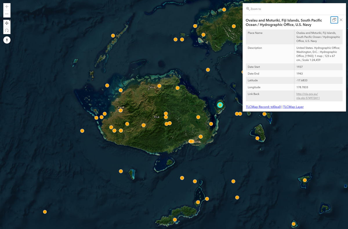
Fig. 30.1 Collection of maps relating to Fiji visualised in GHAP#
Tools and data#
![]()
These datasets contain metadata describing digitised maps in Trove, including geospatial coordinates.
![]()
This notebook helps you create subsets of digitised maps by searching for maps whose centre points fall within a specified bounding box. You can download the results as CSV and GeoJSON files.
![]()
GHAP makes easily available aggregated data on ‘all’ placenames in Australia, including historical names.
Finding digitised maps in Trove#
To find digitised maps in Trove you can use a variation of my standard hack, searching for "nla.obj" in the ‘Image’ category, and then setting ‘Type’ to Maps, ‘Format’ to Map, and ‘Access’ to Online. This search currently returns more that 40,000 results.

But of course the important thing about maps is that they relate to a particular place. How do you find digitised maps in Trove by their location? Trove provides a very broad ‘Place’ facet which lets you filter by state or country, but this is based on text values in the spatial field of the metadata, not on their actual coordinates. The NLA’s Mapsearch interface (which is strangely hidden away) does let you search by spatial coordinates, but it returns less than half the digitised maps I’ve found with coordinates in their metadata and doesn’t let you download a list of results. My own cluster map of digitised map locations is fun to explore, but doesn’t help you create a dataset for further analysis or annotation.
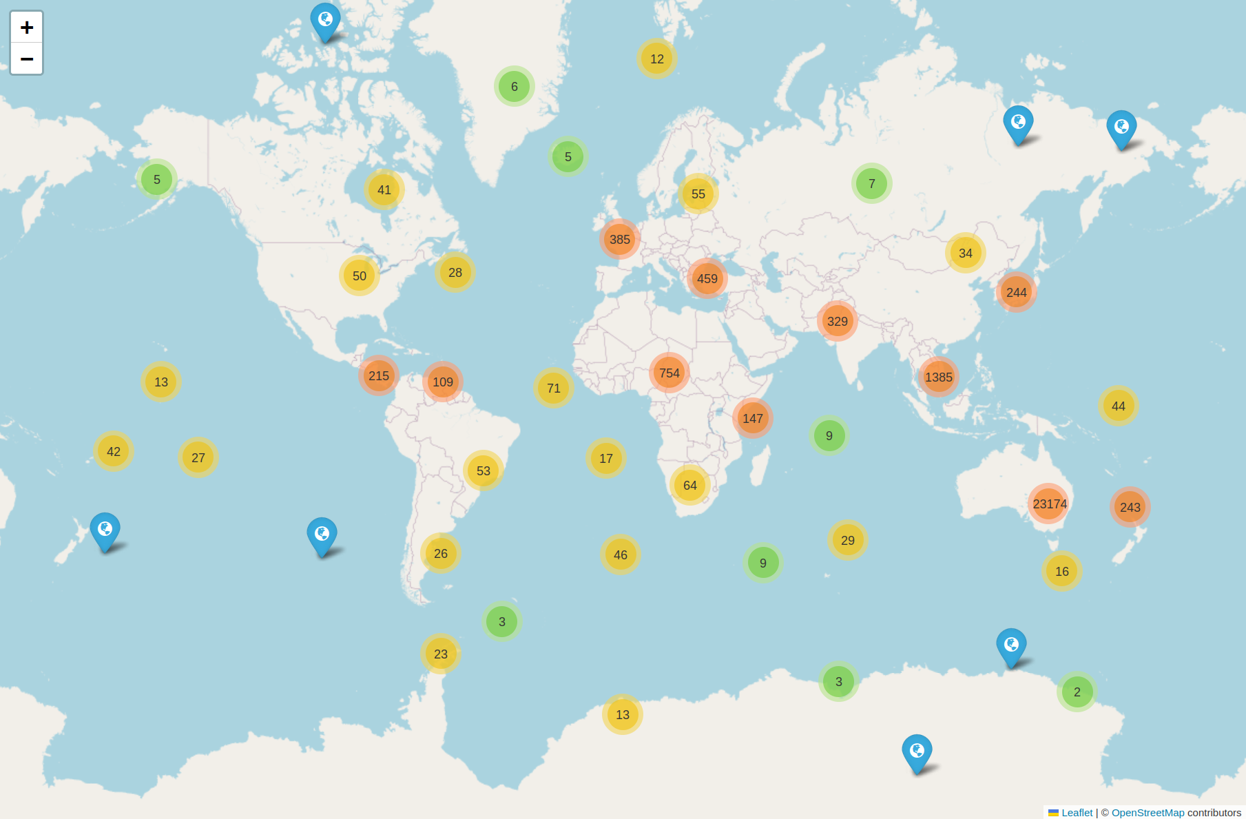
Fig. 30.2 Explore locations of Trove’s digitise maps#
By harvesting data about digitised maps from the Trove API and then enriching the records with metadata embedded in the digitised map viewer, I’ve managed to find 28,205 digitised maps with geospatial coordinates. You can use this data to find maps by their location.
Digitised map metadata and coordinates#
This tutorial uses two related datasets. The first dataset contains data describing digitised maps, harvested from the Trove API and enriched with metadata embedded in the digitised map viewer. This enriched metadata sometimes includes a text string containing spatial information – either the maps centre point, or a bounding box.
The search parameters used to create this dataset were:
"q": '"nla.obj-"',
"category": "image",
"l-artType": "map",
"l-availability": "y",
"l-format": "Map/Single map"
It’s important to note that the format facet was set to Map/Single map, rather than the broader Map. This was to avoid complications with map series which Trove sometimes groups as versions of a single work. But it does mean that a significant amount of maps could be missing from the dataset. A future version will try to work around this issue and include more maps.
The second dataset is the result of an attempt to parse the spatial metadata as geospatial coordinates. Of the 34,844 maps in the initial dataset, 28,205 had usable spatial metadata. For example, the string
(E 130⁰50'--E 131⁰00'/S 12⁰30'--S 12⁰40')
was parsed as:
Type |
Value |
|---|---|
East |
131.000000 |
West |
130.833333 |
North |
-12.500000 |
South |
-12.666667 |
If the spatial metadata described a bounding box, rather than a point, the centre point of the box was also calculated:
Type |
Value |
|---|---|
Latitude |
-12.5833 |
Longitude |
130.9167 |
The spatial metadata includes a significant number of errors and inconsistencies. The parsing process excluded values that were obviously wrong, such as latitudes greater than 90, and changed a small number where latitudes or longitudes had the wrong sign. But other errors remain. Don’t be surprised if maps pop up in unexpected locations. The spatial metadata provides a useful way of exploring and aggregating the digitised maps, but you shouldn’t assume that it is always accurate.
Creating a subset of digitised maps by searching for coordinates#
As noted, 28,205 maps in the harvested dataset have usable spatial coordinates. The GLAM Workbench notebook Create a subset of digitised maps by searching for coordinates uses this data to create a GeoDataFrame that you can query using another set of coordinates. For example, if you query the GeoDataFrame with a bounding box it will return details of all the maps whose centre points fall within the coordinates of that bounding box. In other words, you can find maps by their location.
To make it easier to query by bounding box, the notebook generates a world map showing map locations. You simply use the map’s rectangle drawing tool to select a particular region. The notebook returns details of all maps in that region, providing downloadable datasets in CSV and GeoJSON formats.
Running the notebook#
Go to Create a subset of digitised maps by searching for coordinates in the Trove maps section of the GLAM Workbench.
This notebook, like all GLAM Workbench notebooks, needs to be run in a customised computing environment. The easiest way to do this is through BinderHub. BinderHub is a cloud-based service that gets a notebook up and running by reading its requirements from a code repository, and creating an environment with the necessary software. The GLAM Workbench is integrated with two BinderHub services:
ARDC Binder – based in Australia, requires login using university credentials
MyBinder – international, no login required
If you have a login at an Australian university or research agency, try the ARDC Binder service first. It’s a little more effort, but it’s usually faster and more reliable than the public MyBinder service which can have capacity issues.
The GLAM Workbench displays a preview of the notebook, with options to run it using either the ARDC Binder or MyBinder service.
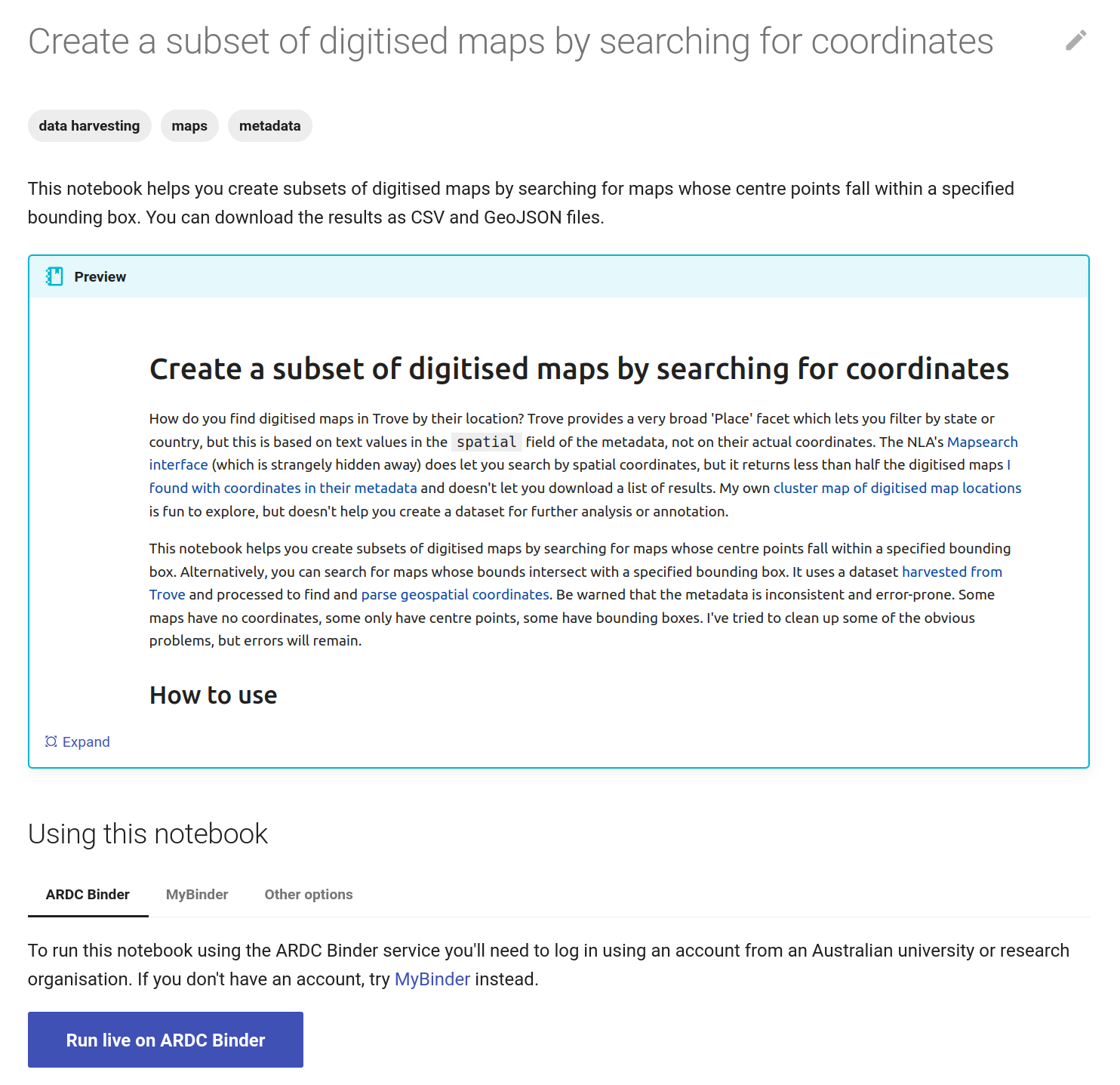
Fig. 30.3 The GLAM Workbench provides a number of ways you can run the notebook#
Using ARDC Binder#
To use the ARDC Binder service, click on the ARDC Binder tab under the notebook preview. You should see a big, blue Run live on ARDC Binder button. Click on the button to launch the Binder service.
If this is the first time you’ve used the ARDC Binder service you’ll be asked to login using the Australian Access Federation (AAF).

Fig. 30.4 ARDC Binder will ask you to log in using AAF#
Click on the Sign in with AAF/Tuakiri button. You’ll be asked to select either AAF or Tuakiri – select AAF.
To sign in with AAF, select your institution from the list, then click the Continue to your organisation button.
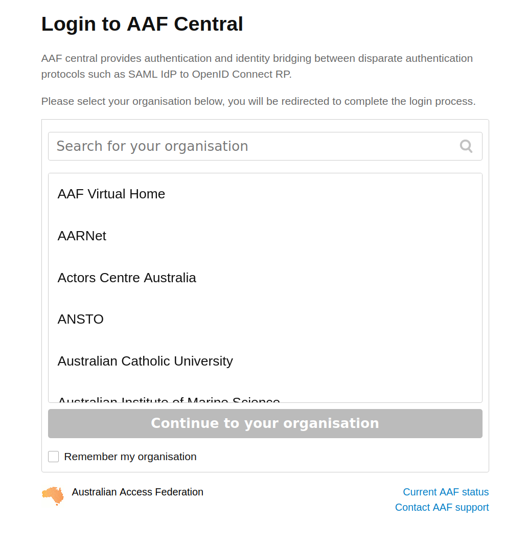
Fig. 30.5 Select your institution from the AAF list#
You’ll be redirected to your insitution’s login screen. Log in using your usual credentials. Once you’ve logged in you’ll be redirected back to ARDC Binder and the notebook will start to load. You might have to wait a bit while a customised computing environment is prepared for you. If you see a message saying that things are taking a long time and there might be a problem, just ignore it. Eventually the notebook will load in the Jupyter Lab interface.
Using MyBinder#

Fig. 30.6 Click on the MyBinder tab#
To use the MyBinder service, click on the MyBinder tab under the notebook preview. You should see a big, blue Run live on MyBinder button. Click on the button to launch the Binder service. No login is required, so MyBinder immediately starts building a customised computing environment. This can take a while, but eventually the notebook should load in the Jupyter Lab interface.
Using the notebook in Jupyter Lab#
No matter what service you use to run the notebook, the result will be the same – the notebook will open in the Jupyter Lab interface.
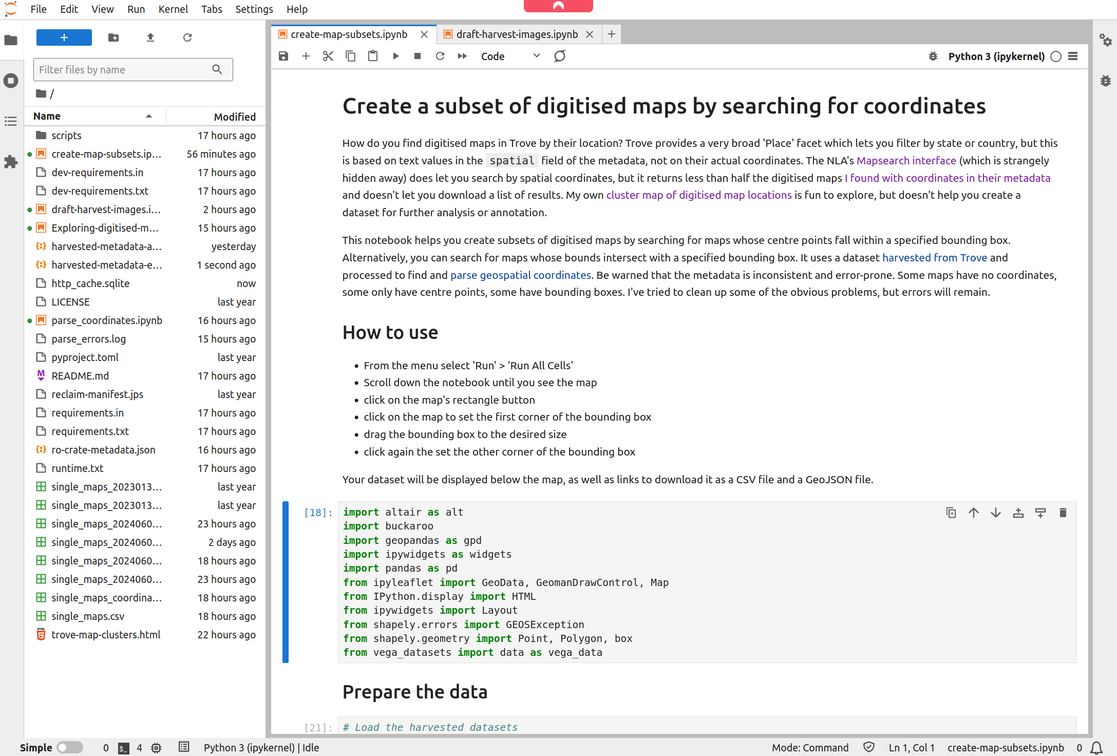
Fig. 30.7 The notebook running in Jupyter Lab#
To generate the map you use to select regions, choose ‘Run All Cells’ from the notebook’s ‘Run’ menu.
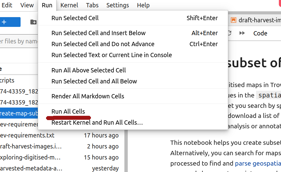
Fig. 30.8 Select Run > Run All Cells from the menu#
Scroll down the the bottom of the notebook and wait for the map to appear. You can move around the map by dragging with your mouse, and zoom in and out using the + and - buttons.
Once you’ve found an area of interest, click on the rectangle drawing button. Click on the map to set the first corner of the bounding box, drag to expand the box, then click again to finish the box and submit your query.
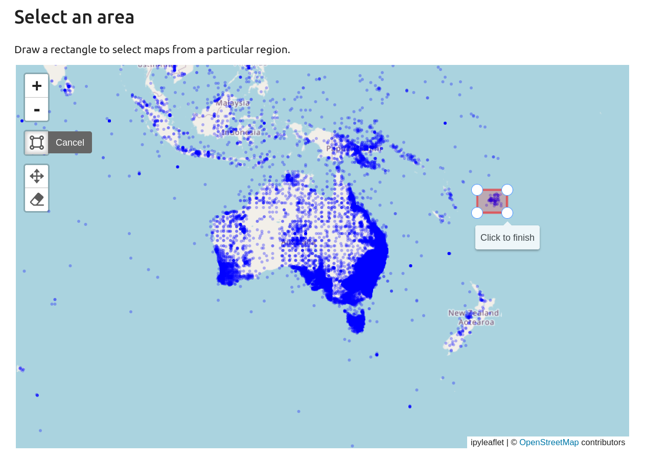
Fig. 30.9 Use the rectangle drawing tool to select an area#
The results of your query will be displayed below the map. You can scroll and sort the list of maps. There’ll also be links to download the dataset, either as a CSV (spreadsheet) or GeoJSON file.
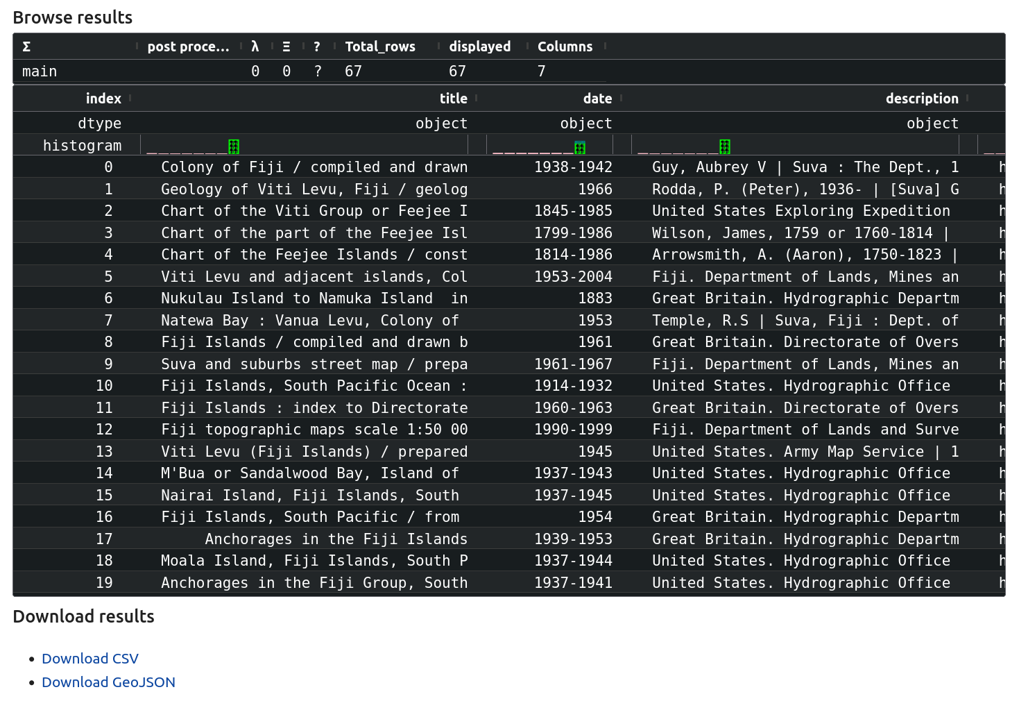
Fig. 30.10 Browse your results and download the dataset as a CSV or GeoJSON file#
Understanding your results#
Both the CSV and GeoJSON files are named according to the coordinates of the bounding box used in the query. So the file named:
174-43359_182-167965_-21-543023_-15-546844.csv
was generated using the coordinates: 174.43359, 182.167965, -21.543023, -15.546844.
The CSV file has been formatted to provide the columns expected by GHAP. These are:
column |
description |
|---|---|
|
map title |
|
earliest year |
|
latest year |
|
combines information on creators, publisher, physical format, and scale |
|
link to view the map in Trove’s digitised map viewer |
|
latitude of map’s centre point |
|
longitude of map’s centre point |
The GeoJSON file includes the full set of spatial coordinates – either a rectangle describing the bounds of the map, or the centre point – as well as the descriptive metadata. GeoJSON is a standard format, so many geospatial data tools will be able to import and use the file. In fact, Jupyter Lab has its own GeoJSON plugin. Find your GeoJSON file in Jupyter Labs file browser and double click it.
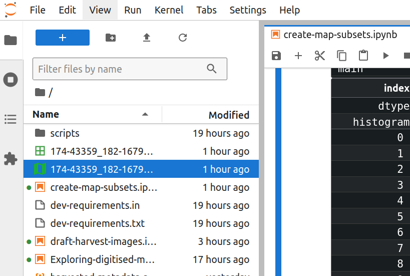
Fig. 30.11 Double click on the GeoJSON file to open it in JupyterLab#
Jupyter Lab will automatically display the map bounds and points on a basemap.
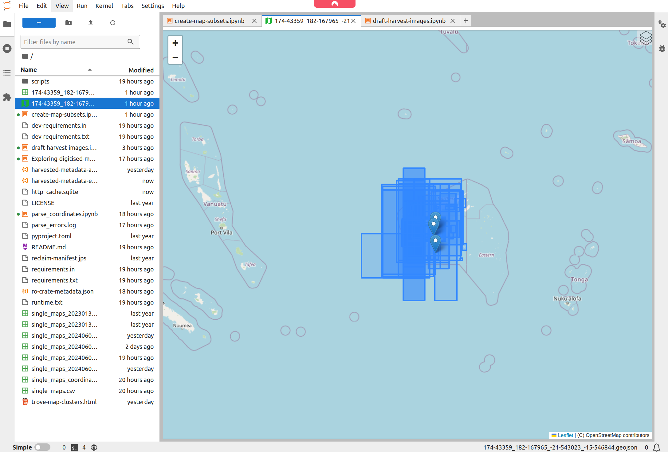
Fig. 30.12 Jupyter Lab displays your GeoJSON data on a map#
Click on the CSV file link to download it to your computer.

Fig. 30.13 Download the CSV file#
Upload your data to a new layer in GHAP#
Now you have a dataset, you can create a layer in GHAP and upload it.
You’ll need a GHAP account to proceed. If you don’t have one click on ‘Login’ and then Register. Fill in the required details and wait for the confirmation email to arrive (mine landed in the spam folder).
Login to your GHAP account.
From the GHAP home page, click on the ‘My Layers’ link.
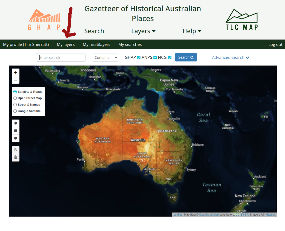
Fig. 30.14 Click on the ‘My Layers’ link#
From the ‘My Layers’ page, click on the Create Layer button.
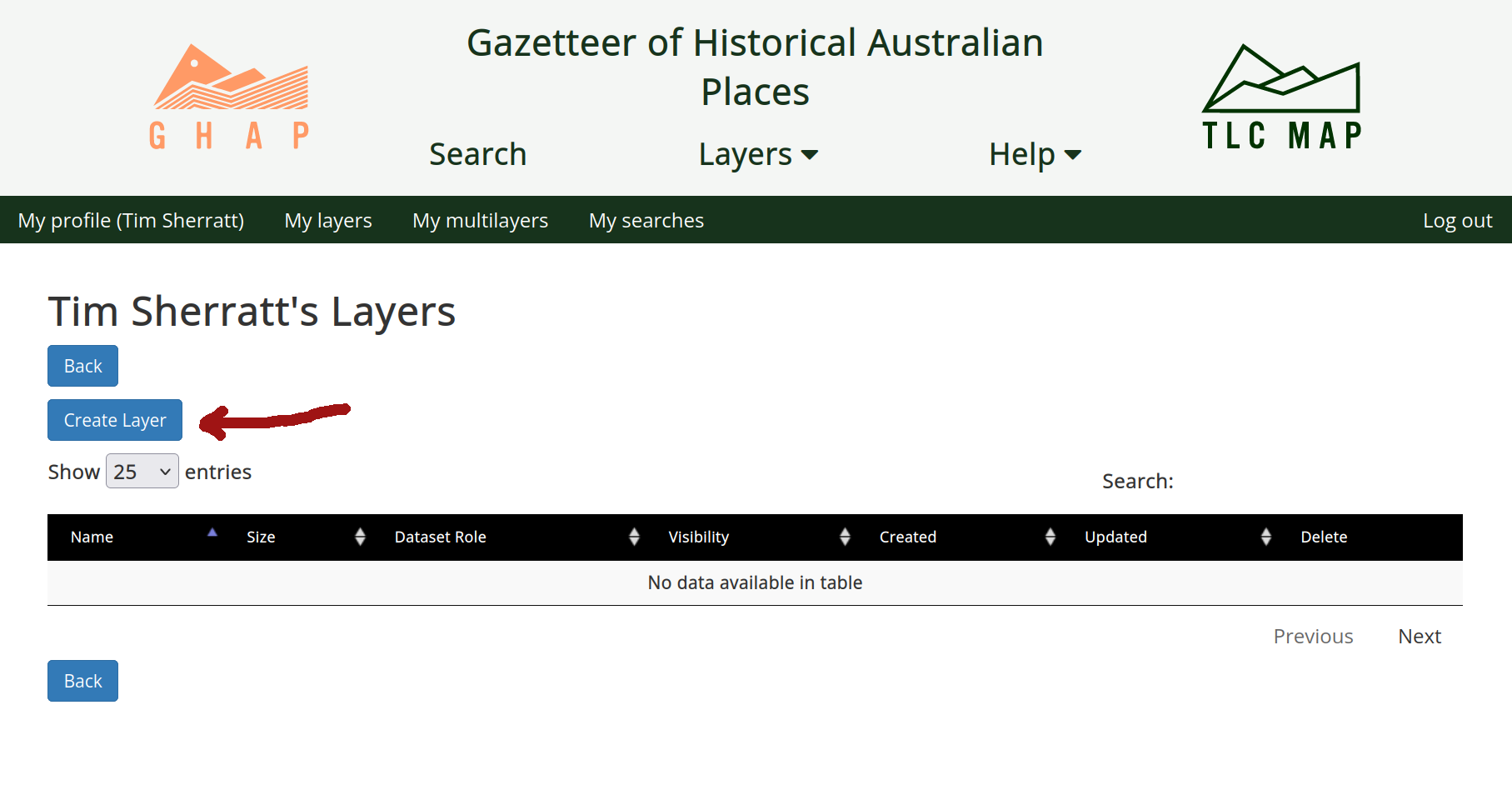
Fig. 30.15 Click on the Create Layer button#
Enter details about your layer into the ‘New Layer’ form. At the very least, you’ll need to supply a ‘Layer name’ and ‘Description’. You can add additional metadata later if you want. When you’ve finished, scroll to the bottom of the form and click on the Create Layer button.
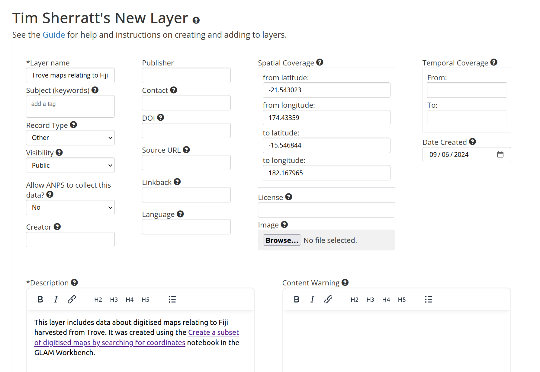
Fig. 30.16 Describe your layer#
You’ll be redirected to a new page displaying the details of your layer. Click on the Import from file button to upload your dataset.
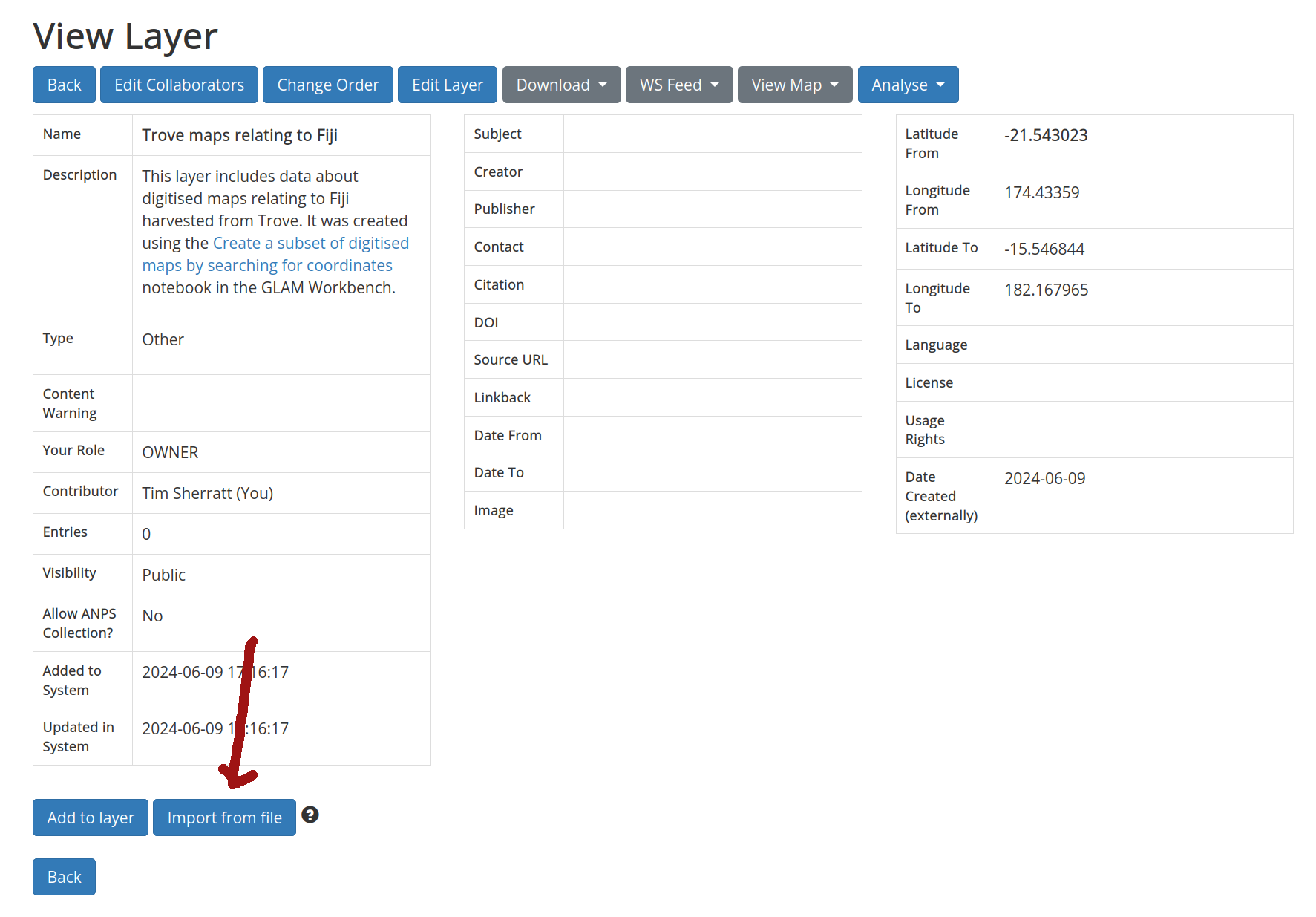
Fig. 30.17 Click on the Import from file button#
Click on the Browse buttom and select the CSV file you downloaded from the notebook. Then click the Upload File button.
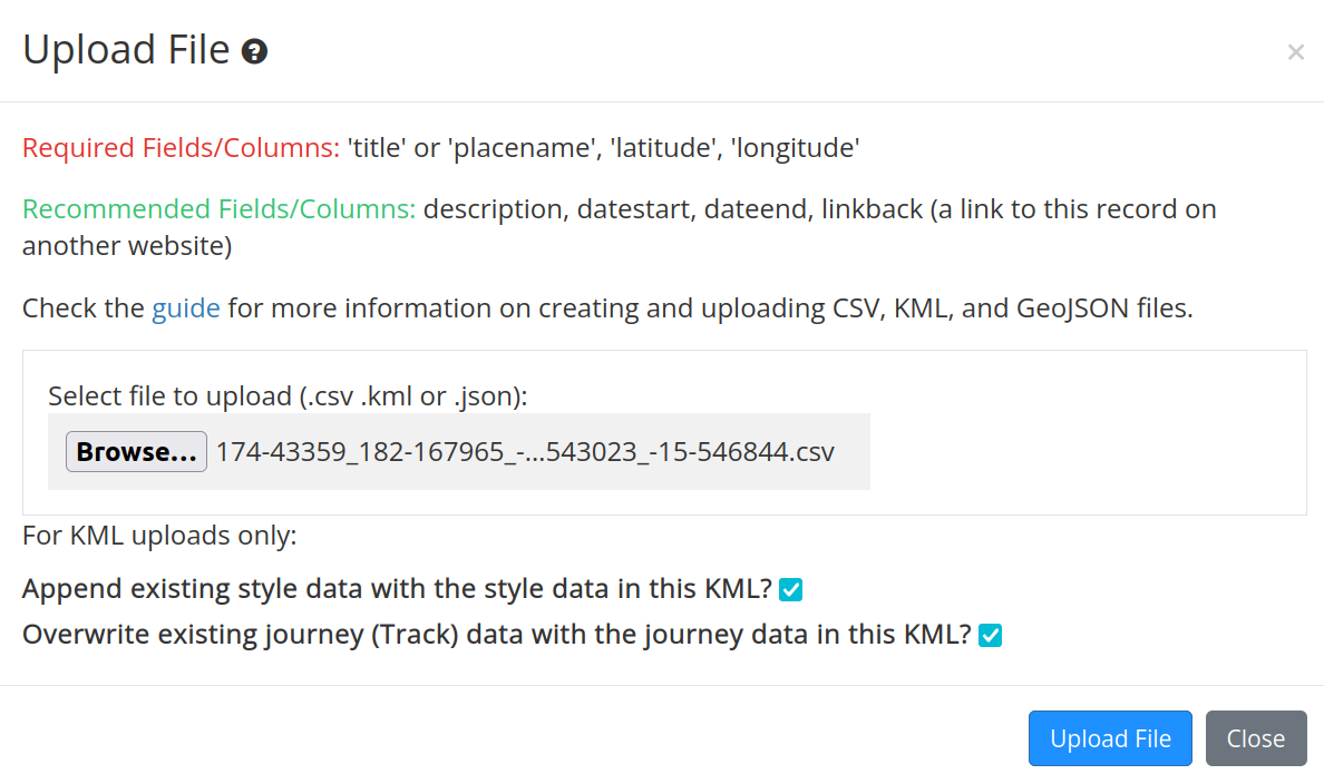
Fig. 30.18 Select and upload the CSV data file#
Metadata from all the digitised maps in your dataset will now be listed on the layer page.
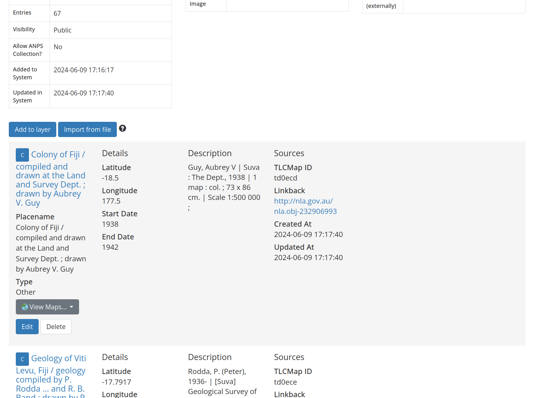
Fig. 30.19 View the uploaded data on the layer page#
At the top of the layer page click on the View Map button and select ‘3D Viewer’ to display your new layer on a map.
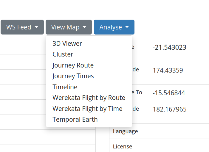
Fig. 30.20 Select ‘3D Viewer’ to display your layer on a map#
A 3D map of the world will load, centred on your data.
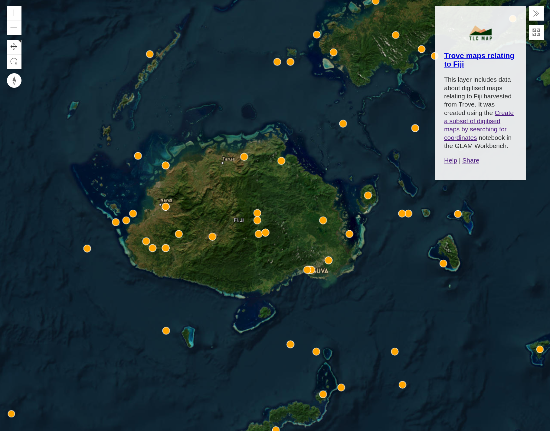
Fig. 30.21 Explore your layer on a 3D map#
Each marker represents a digitised map in your dataset. Click on a marker to display the map’s metadata. To view the digitised map in Trove, click on the ‘Link Back’ url.
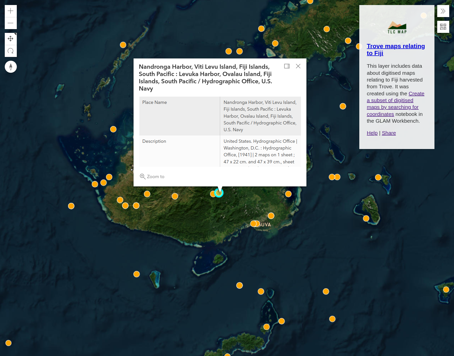
Fig. 30.22 Click on the markers to display map details#
See the GHAP User Guide for more information on sharing and analysing your layer.